EDA is the unstructured process of probing the data we haven’t seen before to understand more about it with a view to thinking about how we can use the data, and to discover what it reveals as insights at first glance.
At other times, we need to analyze some data with no particular objective in mind except to find out if it could be useful for anything at all.
Consider a situation where your manager points you to some data and asks you to do some analysis on it. The data could be in a Google Drive, or a Github repo, or on a thumb drive. It may have been received from a client, a customer or a vendor. You may have a high level pointer to what the data is, for example you may know there is order history data, or invoice data, or web log data. The ask may not be very specific, nor the goal clarified, but we would like to check the data out to see if there is something useful we can do with it.
In other situations, we are looking for something specific, and are looking for the right data to analyze. For example, we may be trying to to identify zip codes where to market our product. We may be able to get data that provides us information on income, consumption, population characteristics etc that could help us with our task. When we receive such data, we would like to find out if it is fit for purpose.
7.2 Inquiries to conduct
So when you get data that you do not know much about in advance, you start with exploratory data analysis, or EDA. Possible inquiries you might like to conduct are:
How much data do we have - number of rows in the data?
How many columns, or fields do we have in the dataset?
Data types - which of the columns appear to be numeric, dates or strings?
Names of the columns, and do they tell us anything?
A visual review of a sample of the dataset
Completeness of the dataset, are missing values obvious? Columns that are largely empty?
Unique values for columns that appear to be categorical, and how many observations of each category?
For numeric columns, the range of values (calculated from min and max values)
Distributions for the different columns, possibly graphed
Correlations between the different columns
Exploratory Data Analysis (EDA) is generally the first activity performed to get a high level understanding of new data. It employs a variety of graphical and summarization techniques to get a ‘sense of the data’.
The purpose of Exploratory Data Analysis is to interrogate the data in an open-minded way with a view to understanding the structure of the data, uncover any prominent themes, identify important variables, detect obvious anomalies, consider missing values, review data types, obtain a visual understanding of the distribution of the data, understand correlations between variables, etc. Not all these things can be discovered during EDA, but these are generally the things we look for when performing EDA.
EDA is unstructured exploration, there is not a defined set of activities you must perform. Generally, you probe the data, and depending upon what you discover, you ask more questions.
AI-Assisted EDA: An increasingly useful complement to traditional EDA is to use a large language model (LLM). Tools like ChatGPT Advanced Data Analysis or Claude can accept a dataset and answer questions in plain English — such as ‘what are the outliers?’ or ‘which variables are most correlated?’. This accelerates initial discovery but does not replace rigorous analysis. A solid understanding of the underlying statistics remains essential to validate the outputs of any AI tool.
7.3 Introduction to Arrays
Arrays, or collection of numbers, are fundamental to analytics at scale. We will cover arrays from a NumPy lens exclusively, given how much NumPy dominates all array based manipulation.
NumPy is the underlying library for manipulating arrays in Python. And arrays are really important for analytics. The reason arrays are important is because many analytical algorithms will only accept arrays as input. Deep learning networks will exclusively accept only arrays as input, though arrays are called tensors in the deep learning world. In addition to this practical issue, data is much easier to manipulate, transform and perform mathematical operations on if it is expressed as an array.
NumPy underpins pandas as well as many other libraries. So we may not be using it a great deal, but there will be situations where numpy is unavoidable.
Below is a high level overview of what arrays are, and some basic array operations.
Modern Alternative — Polars: While NumPy remains foundational and pandas the dominant DataFrame library, Polars has emerged as a high-performance alternative built in Rust. It offers significant speed advantages on large datasets and a clean, expressive API. Install with pip install polars. Deep learning frameworks use the word tensor for arrays; PyTorch tensors and NumPy arrays are conceptually the same thing, and PyTorch provides torch.from_numpy() to convert between them.
7.3.1 Multi-dimensional data
Arrays have structure in the form of dimensions, and numbers sit at the intersection of these dimensions. In a spreadsheet, you see two dimensions - one being the rows, represented as 1, 2, 3…, and the other the columns, repesented as A, B, C. Numpy arrays can have any number of dimensions, even though dimensions beyond the third are humanly impossible to visualize.
A numpy array when printed in Python encloses data for a dimension in square brackets. The fundamental unit of an array of any size is a single one-dimensional row where numbers are separated by commas and enclosed in a set of square brackets, for example, [1, 2, 3, 1]. Several of these will then be arranged within additional nested square brackets to make up the complete array. To understand the idea of an array, mentally visualize a 2-dimensional array similar to a spreadsheet. Every number within the array exists at the intersection of all of its dimensions. In Python, each position along a dimension, more commonly called an axis, is represented by numbers starting with the first element being 0. These positions are called indexes.
The number of square brackets [ gives the number of dimensions in the array. Two are represented on screen, the rows and columns, like a 2D matrix. But the screen is two-dimensional, and cannot display additional dimensions. Therefore all other dimensions appear as repeats of rows and columns - look at the example next. The last two dimensions, eg here 3, 4 represent rows and columns. The 2, the first one, means there are two sets of these rows and columns in the array!
Code
from IPython.display import YouTubeVideo, display, Markdowndisplay(Markdown('**This video provides an introduction to multi-dimensional data, ie, data arrays**'))YouTubeVideo('UsNB7MVl_ds', width=672, height=378)
This video provides an introduction to multi-dimensional data, ie, data arrays
7.3.2 Starting Coding in Python
Next, we will jump into checking things out with code. Let us familiarize ourselves with the Jupyter interface in the next video.
Code
display(Markdown('**Lab exercise - navigating the Jupyter interface**'))YouTubeVideo('57z2j-n29Lo', width=672, height=378)
Lab exercise - navigating the Jupyter interface
7.3.3 Creating arrays with Numpy
Everything that Numpy touches ends as an array, just like everything from a pandas function is a dataframe. Easiest way to generate a random array is np.random.randn(2,3) which will give an array with dimensions 2,3. You can pick any other dimensions too. randn gives random normal numbers.
Code
# import some librariesimport pandas as pdimport osimport randomimport numpy as npimport scipyimport mathimport joblib
The next video provides an introduction to data arrays.
Code
display(Markdown('**Lab exercise - arrays in Python**'))YouTubeVideo('wGJ1z6ucO2U', width=672, height=378)
Lab exercise - arrays in Python
Code
# Create a one dimensional arraynp.random.randn(4)
Numpy axes numbers run from left to right, starting with the index 0. So x.shape gives me 2, 3, 4 which means 2 is the 0th axis, 3 rows are the 1st axis and 4 columns are the 2nd axis.
The shape of the above array is (2, 3, 4)
axis = 0 means : (2, 3, 4)
axis = 1 means : (2, 3, 4)
axis = 2 means : (2, 3, 4)
Code
# Create a 3-dimensional arraydata = np.random.randn(2, 3, 4)print('The shape of the array is:', data.shape)data
The number of [ gives the number of dimensions in the array.
Two are represented on screen, the rows and columns. All others appear afterwards. The last two dimensions, eg here 3, 4 represent rows and columns. The 2, the first one, means there are two sets of these rows and columns in the array.
# Now let us add another dimension. But this time random integers than random normal.# The random integer function (randint) requires specifying low and high for the uniform distribution.data = np.random.randint(low =1, high =100, size = (2,3,2,4))data
# Create an empty array - useful if you need a place to keep data that will be generated later in the code.# It shows zeros but is actually emptynp.empty([2,3])
Putting the axis = n argument with a summarization function (eg, sum) makes the axis n disappear, having been summarized into the function’s results, leaving only the rest of the dimensions. So np.sum(array_name, axis = n), similarly mean(), min(), median(), std() etc will calculate the aggregation function by collapsing all the elements of the selected axis number into one and performing that operation. See below using the sum function.
Code
x = data = np.random.randint(low =1, high =100, size = (2,3))x
array([[97, 53,  5],
       [12, 13, 46]])
Code
# So with axis = 0, the very first dimension, ie the 2 rows, will collapse leaving an array of shape (3,)x.sum(axis =0)
array([109, 66, 51])
Code
# So with axis = 0, the very first dimension, ie the 2 rows, will collapse leaving an array of shape (2,)x.sum(axis =1)
array([155, 71])
7.3.5 Subsetting arrays (‘slices’)
Python starts numbering things starting with zero, which means the first item is the 0th item.
The portion of the dimension you wish to select is given in the form start:finish where the start element is included, but the finish is excluded. So 1:3 means include 1 and 2 but not 3.
Generally, use the above ‘Long Form’ way for slicing where you specify the indices for each dimension. Where everything is to be included, use :. There are other short-cut methods of slicing, but can leave those as is.
Imagine an array a1 with dimensions (3, 5, 2, 4). This means: - This array has 3 arrays in it that have the dimensions (5, 2, 4) - Each of these 3 arrays have 5 additional arrays each in them of the dimension (2,4). (So there are 3*5=15 of these 2x4 arrays) - Each of these (2,4) arrays has 2 one-dimensional arrays with 4 columns.
If in the slice notation only a portion of what to include is specified, eg a1[0], then it means we are asking for the first one of these axes, ie the dimension parameters are specifying from the left of (3, 5, 2, 4). It means give me the first of the 3 arrays with size (5,2,4).
If the slice notation says a1[0,1], then it means 0th element of the first dim, and 1st element of the second dim.
# Select subset of named rows and columnsa1[[0, 3]][:,[0, 1]] # Named rows and columns. # Note that a1[[0, 3],[0, 1]] does not work as expected, it selects two points (0,0)and (3,1). # Really crazy but it is what it is.
array([[90, 63],
       [63, 79]])
### Operations on arrays All math on arrays is element wise, and scalars are multiplied/added with each element.
np.sum(array1) # adds all the elements of an array
761
Code
np.sum(array1, axis =0) # adds all elements of the array along a particular axis
array([119, 127, 167, 140, 208])
7.3.7 Matrix math
Numpy has arrays as well as matrices. Matrices are 2D, arrays can have any number of dimensions. The only real difference between a matrix (type = numpy.matrix) and an array (type = numpy.ndarray) is that all array operations are element wise, ie the special R x C matrix multiplication does not apply to arrays. However, for an array that is 2 x 2 in shape you can use the @ operator to do matrix math.
So that leaves matrices and arrays interchangeable in a practical sense. Except that you can’t do an inverse of an array using .I which you can for a matrix.
Code
import warnings as _w_w.filterwarnings('ignore', category=PendingDeprecationWarning, message='.*matrix subclass.*') # intentional demo section# NOTE: np.matrix is deprecated since NumPy 1.15. Prefer np.array throughout.# For matrix multiply use the @ operator; for inverse use np.linalg.inv(a)# Create a matrix 'm' and an array 'a' that are identicalm = np.matrix(np.random.randint(0,10,(3,3)))a = np.array(m)
For np.matrix objects, * performs matrix multiplication (but np.matrix is deprecated — prefer np.array with @ for all new code). If using arrays, use @ for matrix multiplication, which also works for matrices. So just to be safe, just use @.
Dot-product is the same as row-by-column matrix multiplication, and is not elementwise.
Used for calculating the inverse of a matrix, and only applies to square matrices.
Code
np.linalg.det(m)
308.0000000000001
7.3.7.7 Converting from matrix to array and vice-versa
np.asmatrix and np.asarray allow you to convert one to the other. Though above we have just used np.array and np.matrix without any issue.
The above references: https://stackoverflow.com/questions/4151128/what-are-the-differences-between-numpy-arrays-and-matrices-which-one-should-i-u
7.3.7.8 Distances and angles between vectors
Size of a vector, angle between vectors, distance between vectors
Code
# We set up two vectors a and ba = np.array([1,2,3]); b = np.array([5,4,3])print('a =',a)print('b =',b)
a = [1 2 3]
b = [5 4 3]
Code
# Size of the vector, computed as the root of the squares of each of the elementsnp.linalg.norm(a)
3.7416573867739413
Code
# Distance between two vectorsnp.linalg.norm(a - b)
4.47213595499958
Code
# Which is the same as print(np.sqrt(np.dot(a, a) -2* np.dot(a, b) + np.dot(b, b)))(a@a + b@b -2*a@b)**.5
4.47213595499958
4.47213595499958
Code
# Combine the two vectorsX = np.concatenate((a,b)).reshape(2,3)X
array([[1, 2, 3],
       [5, 4, 3]])
Code
# Euclidean distance is the default metric for this function# from sklearnfrom sklearn.metrics import pairwise_distancespairwise_distances(X)
array([[0.        , 4.47213595],
       [4.47213595, 0.        ]])
Code
# Angle in radians between two vectors. To get the# answer in degrees, multiply by 180/pi, or 180/math.pi (after import math). Also there is a function in math called# math.radians to get radians from degrees, or math.degrees(x) to convert angle x from radians to degrees.import mathangle_in_radians = np.arccos(np.dot(a,b) / (np.linalg.norm(a) * np.linalg.norm(b))) angle_in_degrees = math.degrees(angle_in_radians)print('Angle in degrees =', angle_in_degrees)print('Angle in radians =', angle_in_radians)
Angle in degrees = 33.74461333141198
Angle in radians = 0.5889546074455115
Code
# Same as above using math.acos instead of np.arccosmath.acos(np.dot(a,b) / (np.linalg.norm(a) * np.linalg.norm(b)))
0.5889546074455115
7.3.7.9 Sorting with argsort
Which is the same as sort, but shows index numbers instead of the values
Code
# We set up an arraya = np.array([20,10,30,0])
Code
# Sorted indicesnp.argsort(a)
array([3, 1, 0, 2], dtype=int64)
Code
# Using the indices to get the sorted valuesa[np.argsort(a)]
array([ 0, 10, 20, 30])
Code
# Descending sort indicesnp.argsort(a)[::-1]
array([2, 0, 1, 3], dtype=int64)
Code
# Descending sort valuesa[np.argsort(a)[::-1]]
array([30, 20, 10, 0])
7.4 Understanding DataFrames
As we discussed in the prior section, understanding and manipulating arrays of numbers is fundamental to the data science process. This is because nearly all ML and AI algorithms insist on being provided data arrays as inputs, and the NumPy library underpins almost all of data science.
As we discussed, a NumPy array is essentially a collection of numbers. This collection is organized along ‘dimensions’. So NumPy objects are n-dimensional array objects, or ndarray, a fast and efficient container for large datasets in Python.
But arrays have several limitations. One huge limitation is that they are raw containers with numbers, they don’t have ‘headers’, or labels that describe the columns, rows, or the additional dimensions. This means we need to track separately somewhere what each of the dimensions mean. Another limitation is that after 3 dimensions, the additional dimensions are impossible toto visualize in the human mind. For most practical purposes, humans like to think of data in the tabular form, with just rows and columns. If there are more dimensions, one can have multiple tables.
This is where pandas steps in. Pandas use dataframes, or a spreadsheet like construct where there are rows and columns, and these rows and columns can have names or headings. Pandas dataframes are easily converted to NumPy arrays, and algorithms will mostly accept a dataframe as an input just as they would an array.
7.4.1 Exploring Tabular Data with Pandas
Tabular data is often the most common data type that is encountered, though ‘unstructured’ data is increasingly becoming common. Tabular data is two dimensional data – with rows and columns. The columns are defined and understood, and we generally understand what they contain.
Data is laid out as a 2-dimensional matrix, whether in a spreadsheet, or R/Python dataframes, or in a database table.
Rows generally represent individual observations, while columns are the fields/variables.
Variables can be numeric, or categorical.
Numerical variables can be integers, floats etc, and are continuous.
Categorical variables may be cardinal (eg, species, gender), or ordinal (eg, low, medium, high), and belong to a discrete set.
Categorical variables are also called factors, and levels.
Algorithms often require categorical variables to be converted to numerical variables.
Unstructured data includes audio, video and other kinds of data that is useful for problems of perception. Unstructured data will almost invariably need to be converted into structured arrays with defined dimensions, but for the moment we will skip that.
7.4.2 Reading data with Pandas
Pandas offer several different functions for reading different types of data. > read_csv : Load comma separated files
> read_table : Load tab separated files
> read_fwf : Read data in fixed-width column format (i.e., no delimiters)
> read_clipboard Read data from the clipboard; useful for converting tables from web pages
> read_excel : Read Excel files
> read_html : Read all tables found in the given HTML document
> read_json : Read data from a JSON (JavaScript Object Notation) file
> read_pickle : Read a pickle file
> read_sql : Read results of an SQL query
> read_sas : Read SAS files
pandas 2.0 — Copy-on-Write (2023): pandas 2.0 introduced Copy-on-Write semantics. Chained assignment like df[df.x > 1]['y'] = 0 will produce a SettingWithCopyWarning and may silently fail. Always use df.loc[condition, column] = value for safe, explicit assignment. See pandas 2.0 migration guide for details.
7.5 Other data types in Python
Lists are represented as []. Lists are a changeable collection of elements, and the elements can be any Python data, eg strings, numbers, dictionaries, or even other lists.
Dictionaries are enclosed in {}. These are ‘key:value’ pairs, where ‘key’ is almost like a name given to a ‘value’.
Sets are also enclosed in {}, except they don’t have the colons separating the key:value pairs. These are collections of items, and they are unordered.
Tuples are collections of variables, and enclosed in (). They are different from sets in that they are unchangeable.
Next is a quick video covering data types relevant to data analysis.
Code
display(Markdown('**Lab exercise - other data types we should know about**'))YouTubeVideo('Tr7J03-GUq0', width=672, height=378)
Lab exercise - other data types we should know about
Code
# Example - creating a listempty_list = []list1 = ['a', 2,4, 'python']list1
['a', 2, 4, 'python']
Code
# Example - creating a dictionarydict1 = {'first': ['John', 'Jane'], 'something_else': (1,2,3)}dict1
Before we move forward with getting into the details with EDA, we will first take a small digressive detour to talk about data sets.
In order to experiment with EDA, we need some data. We can bring our own data, but for exploration and experimentation, it is often easy to load up one of the many in-built datasets accessible through Python. These datasets cover the spectrum - from really small datasets to those with many thousands of records, and include text data such as movie reviews and tweets.
We will leverage these built in datasets for the rest of the discussion as they provide a good path to creating reproducible examples. These datasets are great for experimenting, testing, doing tutorials and exercises.
The next few headings will cover these in-built datasets.
The Statsmodels library provides access to several interesting inbuilt datasets in Python.
The datasets available in R can also be accessed through statsmodels.
The Seaborn library has several toy datasets available to explore.
The Scikit Learn (sklearn) library also has in-built datasets.
Scikit Learn also provides a function to generate random datasets with described characteristics (make_blobs function)
In the rest of this discussion, we will use these data sets and explore the data.
Some of these are described below, together with information on how to access and use such datasets.
Code
# Load the regular librariesimport pandas as pdimport numpy as npimport seaborn as snsimport matplotlib.pyplot as plt
7.6.1 Loading data from Statsmodels
Statsmodels allows access to several datasets for use in examples, model testing, tutorials, testing functions etc. These can be accessed using sm.datasets.macrodata.load_pandas()['data'], where macrodata is just one example of a dataset. Pressing TAB after sm.datasets should bring up a pick-list of datasets to choose from.
The commands print(sm.datasets.macrodata.DESCRLONG) and print(sm.datasets.macrodata.NOTE) provide additional details on the datasets.
Code
# Load macro economic data from Statsmodelsimport statsmodels.api as smdf = sm.datasets.macrodata.load_pandas()['data']df
year
quarter
realgdp
realcons
realinv
realgovt
realdpi
cpi
m1
tbilrate
unemp
pop
infl
realint
0
1959.0
1.0
2710.349
1707.4
286.898
470.045
1886.9
28.980
139.7
2.82
5.8
177.146
0.00
0.00
1
1959.0
2.0
2778.801
1733.7
310.859
481.301
1919.7
29.150
141.7
3.08
5.1
177.830
2.34
0.74
2
1959.0
3.0
2775.488
1751.8
289.226
491.260
1916.4
29.350
140.5
3.82
5.3
178.657
2.74
1.09
3
1959.0
4.0
2785.204
1753.7
299.356
484.052
1931.3
29.370
140.0
4.33
5.6
179.386
0.27
4.06
4
1960.0
1.0
2847.699
1770.5
331.722
462.199
1955.5
29.540
139.6
3.50
5.2
180.007
2.31
1.19
...
...
...
...
...
...
...
...
...
...
...
...
...
...
...
198
2008.0
3.0
13324.600
9267.7
1990.693
991.551
9838.3
216.889
1474.7
1.17
6.0
305.270
-3.16
4.33
199
2008.0
4.0
13141.920
9195.3
1857.661
1007.273
9920.4
212.174
1576.5
0.12
6.9
305.952
-8.79
8.91
200
2009.0
1.0
12925.410
9209.2
1558.494
996.287
9926.4
212.671
1592.8
0.22
8.1
306.547
0.94
-0.71
201
2009.0
2.0
12901.504
9189.0
1456.678
1023.528
10077.5
214.469
1653.6
0.18
9.2
307.226
3.37
-3.19
202
2009.0
3.0
12990.341
9256.0
1486.398
1044.088
10040.6
216.385
1673.9
0.12
9.6
308.013
3.56
-3.44
203 rows × 14 columns
Code
# Print the description of the dataprint(sm.datasets.macrodata.DESCRLONG)
US Macroeconomic Data for 1959Q1 - 2009Q3
Code
# Print the data-dictionary for the different columns/fields in the data

print(sm.datasets.macrodata.NOTE)
::
    Number of Observations - 203

    Number of Variables - 14

    Variable name definitions::

        year      - 1959q1 - 2009q3
        quarter   - 1-4
        realgdp   - Real gross domestic product (Bil. of chained 2005 US$,
                    seasonally adjusted annual rate)
        realcons  - Real personal consumption expenditures (Bil. of chained
                    2005 US$, seasonally adjusted annual rate)
        realinv   - Real gross private domestic investment (Bil. of chained
                    2005 US$, seasonally adjusted annual rate)
        realgovt  - Real federal consumption expenditures & gross investment
                    (Bil. of chained 2005 US$, seasonally adjusted annual rate)
        realdpi   - Real private disposable income (Bil. of chained 2005
                    US$, seasonally adjusted annual rate)
        cpi       - End of the quarter consumer price index for all urban
                    consumers: all items (1982-84 = 100, seasonally adjusted).
        m1        - End of the quarter M1 nominal money stock (Seasonally
                    adjusted)
        tbilrate  - Quarterly monthly average of the monthly 3-month
                    treasury bill: secondary market rate
        unemp     - Seasonally adjusted unemployment rate (%)
        pop       - End of the quarter total population: all ages incl. armed
                    forces over seas
        infl      - Inflation rate (ln(cpi_{t}/cpi_{t-1}) * 400)
        realint   - Real interest rate (tbilrate - infl)
7.6.2 Importing R datasets using Statsmodels
Datasets available in R can also be imported using the command sm.datasets.get_rdataset('mtcars').data, where mtcards can be replaced by the appropriate dataset name.
Code
# Import the mtcars dataset which contains attributes for 32 models of carsmtcars = sm.datasets.get_rdataset('mtcars').data
# Load the diamonds datasetdiamonds = sns.load_dataset('diamonds')
Code
diamonds.head(20)
carat
cut
color
clarity
depth
table
price
x
y
z
0
0.23
Ideal
E
SI2
61.5
55.0
326
3.95
3.98
2.43
1
0.21
Premium
E
SI1
59.8
61.0
326
3.89
3.84
2.31
2
0.23
Good
E
VS1
56.9
65.0
327
4.05
4.07
2.31
3
0.29
Premium
I
VS2
62.4
58.0
334
4.20
4.23
2.63
4
0.31
Good
J
SI2
63.3
58.0
335
4.34
4.35
2.75
5
0.24
Very Good
J
VVS2
62.8
57.0
336
3.94
3.96
2.48
6
0.24
Very Good
I
VVS1
62.3
57.0
336
3.95
3.98
2.47
7
0.26
Very Good
H
SI1
61.9
55.0
337
4.07
4.11
2.53
8
0.22
Fair
E
VS2
65.1
61.0
337
3.87
3.78
2.49
9
0.23
Very Good
H
VS1
59.4
61.0
338
4.00
4.05
2.39
10
0.30
Good
J
SI1
64.0
55.0
339
4.25
4.28
2.73
11
0.23
Ideal
J
VS1
62.8
56.0
340
3.93
3.90
2.46
12
0.22
Premium
F
SI1
60.4
61.0
342
3.88
3.84
2.33
13
0.31
Ideal
J
SI2
62.2
54.0
344
4.35
4.37
2.71
14
0.20
Premium
E
SI2
60.2
62.0
345
3.79
3.75
2.27
15
0.32
Premium
E
I1
60.9
58.0
345
4.38
4.42
2.68
16
0.30
Ideal
I
SI2
62.0
54.0
348
4.31
4.34
2.68
17
0.30
Good
J
SI1
63.4
54.0
351
4.23
4.29
2.70
18
0.30
Good
J
SI1
63.8
56.0
351
4.23
4.26
2.71
19
0.30
Very Good
J
SI1
62.7
59.0
351
4.21
4.27
2.66
Code
# Load the mpg dataset from Seaborn. This is similar to the mtcars dataset,# but has a higher count of observations.sns.load_dataset('mpg')
mpg
cylinders
displacement
horsepower
weight
acceleration
model_year
origin
name
0
18.0
8
307.0
130.0
3504
12.0
70
usa
chevrolet chevelle malibu
1
15.0
8
350.0
165.0
3693
11.5
70
usa
buick skylark 320
2
18.0
8
318.0
150.0
3436
11.0
70
usa
plymouth satellite
3
16.0
8
304.0
150.0
3433
12.0
70
usa
amc rebel sst
4
17.0
8
302.0
140.0
3449
10.5
70
usa
ford torino
...
...
...
...
...
...
...
...
...
...
393
27.0
4
140.0
86.0
2790
15.6
82
usa
ford mustang gl
394
44.0
4
97.0
52.0
2130
24.6
82
europe
vw pickup
395
32.0
4
135.0
84.0
2295
11.6
82
usa
dodge rampage
396
28.0
4
120.0
79.0
2625
18.6
82
usa
ford ranger
397
31.0
4
119.0
82.0
2720
19.4
82
usa
chevy s-10
398 rows × 9 columns
Code
# Look at how many cars from each country in the mpg datasetsns.load_dataset('mpg').origin.value_counts()
origin
usa       249
japan      79
europe     70
Name: count, dtype: int64
Code
# Build a histogram of the model yearsns.load_dataset('mpg').model_year.astype('category').hist();
Code
# Create a random dataframe with random datan =25df = pd.DataFrame( {'state': list(np.random.choice(["New York", "Florida", "California"], size=(n))), 'gender': list(np.random.choice(["Male", "Female"], size=(n), p=[.4, .6])),'education': list(np.random.choice(["High School", "Undergrad", "Grad"], size=(n))),'housing': list(np.random.choice(["Rent", "Own"], size=(n))), 'height': list(np.random.randint(140,200,n)),'weight': list(np.random.randint(100,150,n)),'income': list(np.random.randint(50,250,n)),'computers': list(np.random.randint(0,6,n)) })
Code
df
state
gender
education
housing
height
weight
income
computers
0
Florida
Male
Grad
Own
183
108
117
3
1
Florida
Male
Undergrad
Own
154
147
82
3
2
Florida
Male
Grad
Rent
170
142
149
5
3
Florida
Female
High School
Rent
196
115
145
5
4
California
Female
High School
Rent
186
122
212
3
5
New York
Female
Grad
Own
182
141
158
1
6
Florida
Male
Grad
Rent
199
137
124
2
7
California
Female
High School
Rent
189
108
105
3
8
California
Female
High School
Rent
140
132
121
4
9
California
Male
Undergrad
Own
155
116
51
0
10
Florida
Male
Grad
Own
182
132
132
2
11
Florida
Female
Undergrad
Own
157
114
241
3
12
Florida
Female
Undergrad
Rent
150
120
156
3
13
California
Male
Undergrad
Own
170
115
186
2
14
New York
Male
Grad
Own
179
135
157
0
15
California
Male
Undergrad
Own
164
105
215
0
16
Florida
Female
Undergrad
Rent
194
111
128
5
17
New York
Male
High School
Rent
156
134
74
0
18
Florida
Female
High School
Own
141
104
59
2
19
New York
Female
High School
Own
197
149
167
4
20
Florida
Female
High School
Rent
162
142
160
2
21
New York
Male
Grad
Rent
142
118
180
0
22
California
Male
High School
Rent
149
142
124
2
23
Florida
Male
High School
Rent
190
101
55
1
24
California
Male
Grad
Own
140
106
86
5
Code
# Load the 'Old Faithful' eruption datasns.load_dataset('geyser')
duration
waiting
kind
0
3.600
79
long
1
1.800
54
short
2
3.333
74
long
3
2.283
62
short
4
4.533
85
long
...
...
...
...
267
4.117
81
long
268
2.150
46
short
269
4.417
90
long
270
1.817
46
short
271
4.467
74
long
272 rows × 3 columns
7.6.4 Datasets in sklearn
Scikit Learn has several datasets that are built-in as well that can be used to experiment with functions and algorithms. Some are listed below:
Removed in sklearn 1.2:load_boston was permanently removed in December 2022 due to ethical concerns about the dataset. Use fetch_california_housing() as a drop-in replacement:
from sklearn.datasets import fetch_california_housingdata = fetch_california_housing()X, y = data.data, data.target
load_iris(*[, return_X_y, as_frame]) Load and return the iris dataset (classification). load_diabetes(*[, return_X_y, as_frame]) Load and return the diabetes dataset (regression). load_digits(*[, n_class, return_X_y, as_frame]) Load and return the digits dataset (classification). load_linnerud(*[, return_X_y, as_frame]) Load and return the physical excercise linnerud dataset. load_wine(*[, return_X_y, as_frame]) Load and return the wine dataset (classification). load_breast_cancer(*[, return_X_y, as_frame]) Load and return the breast cancer wisconsin dataset (classification).
Let us import the wine dataset next, and the California housing datset after that.
# Let us look at the DESCR for the dataframe we just loadedprint(DESCR)
.. _wine_dataset:

Wine recognition dataset
------------------------

**Data Set Characteristics:**

:Number of Instances: 178
:Number of Attributes: 13 numeric, predictive attributes and the class
:Attribute Information:
    - Alcohol
    - Malic acid
    - Ash
    - Alcalinity of ash
    - Magnesium
    - Total phenols
    - Flavanoids
    - Nonflavanoid phenols
    - Proanthocyanins
    - Color intensity
    - Hue
    - OD280/OD315 of diluted wines
    - Proline
    - class:
        - class_0
        - class_1
        - class_2

:Summary Statistics:

============================= ==== ===== ======= =====
                                Min   Max   Mean     SD
============================= ==== ===== ======= =====
Alcohol:                      11.0  14.8    13.0   0.8
Malic Acid:                   0.74  5.80    2.34  1.12
Ash:                          1.36  3.23    2.36  0.27
Alcalinity of Ash:            10.6  30.0    19.5   3.3
Magnesium:                    70.0 162.0    99.7  14.3
Total Phenols:                0.98  3.88    2.29  0.63
Flavanoids:                   0.34  5.08    2.03  1.00
Nonflavanoid Phenols:         0.13  0.66    0.36  0.12
Proanthocyanins:              0.41  3.58    1.59  0.57
Colour Intensity:              1.3  13.0     5.1   2.3
Hue:                          0.48  1.71    0.96  0.23
OD280/OD315 of diluted wines: 1.27  4.00    2.61  0.71
Proline:                       278  1680     746   315
============================= ==== ===== ======= =====

:Missing Attribute Values: None
:Class Distribution: class_0 (59), class_1 (71), class_2 (48)
:Creator: R.A. Fisher
:Donor: Michael Marshall (MARSHALL%PLU@io.arc.nasa.gov)
:Date: July, 1988

This is a copy of UCI ML Wine recognition datasets.
https://archive.ics.uci.edu/ml/machine-learning-databases/wine/wine.data

The data is the results of a chemical analysis of wines grown in the same
region in Italy by three different cultivators. There are thirteen different
measurements taken for different constituents found in the three types of
wine.

Original Owners:

Forina, M. et al, PARVUS -
An Extendible Package for Data Exploration, Classification and Correlation.
Institute of Pharmaceutical and Food Analysis and Technologies,
Via Brigata Salerno, 16147 Genoa, Italy.

Citation:

Lichman, M. (2013). UCI Machine Learning Repository
[https://archive.ics.uci.edu/ml]. Irvine, CA: University of California,
School of Information and Computer Science.

|details-start|
**References**
|details-split|

(1) S. Aeberhard, D. Coomans and O. de Vel,
Comparison of Classifiers in High Dimensional Settings,
Tech. Rep. no. 92-02, (1992), Dept. of Computer Science and Dept. of
Mathematics and Statistics, James Cook University of North Queensland.
(Also submitted to Technometrics).

The data was used with many others for comparing various
classifiers. The classes are separable, though only RDA
has achieved 100% correct classification.
(RDA : 100%, QDA 99.4%, LDA 98.9%, 1NN 96.1% (z-transformed data))
(All results using the leave-one-out technique)

(2) S. Aeberhard, D. Coomans and O. de Vel,
"THE CLASSIFICATION PERFORMANCE OF RDA"
Tech. Rep. no. 92-01, (1992), Dept. of Computer Science and Dept. of
Mathematics and Statistics, James Cook University of North Queensland.
(Also submitted to Journal of Chemometrics).

|details-end|
Code
# California housing dataset. medv is the median value of the homesfrom sklearn import datasetsX = datasets.fetch_california_housing()['data']y = datasets.fetch_california_housing()['target']features = datasets.fetch_california_housing()['feature_names']DESCR = datasets.fetch_california_housing()['DESCR']cali_df = pd.DataFrame(X, columns = features)cali_df.insert(0,'medv', y)cali_df
medv
MedInc
HouseAge
AveRooms
AveBedrms
Population
AveOccup
Latitude
Longitude
0
4.526
8.3252
41.0
6.984127
1.023810
322.0
2.555556
37.88
-122.23
1
3.585
8.3014
21.0
6.238137
0.971880
2401.0
2.109842
37.86
-122.22
2
3.521
7.2574
52.0
8.288136
1.073446
496.0
2.802260
37.85
-122.24
3
3.413
5.6431
52.0
5.817352
1.073059
558.0
2.547945
37.85
-122.25
4
3.422
3.8462
52.0
6.281853
1.081081
565.0
2.181467
37.85
-122.25
...
...
...
...
...
...
...
...
...
...
20635
0.781
1.5603
25.0
5.045455
1.133333
845.0
2.560606
39.48
-121.09
20636
0.771
2.5568
18.0
6.114035
1.315789
356.0
3.122807
39.49
-121.21
20637
0.923
1.7000
17.0
5.205543
1.120092
1007.0
2.325635
39.43
-121.22
20638
0.847
1.8672
18.0
5.329513
1.171920
741.0
2.123209
39.43
-121.32
20639
0.894
2.3886
16.0
5.254717
1.162264
1387.0
2.616981
39.37
-121.24
20640 rows × 9 columns
Code
# Again, we can look at what the various columns meanprint(DESCR)
.. _california_housing_dataset:

California Housing dataset
--------------------------

**Data Set Characteristics:**

:Number of Instances: 20640

:Number of Attributes: 8 numeric, predictive attributes and the target

:Attribute Information:
    - MedInc        median income in block group
    - HouseAge      median house age in block group
    - AveRooms      average number of rooms per household
    - AveBedrms     average number of bedrooms per household
    - Population    block group population
    - AveOccup      average number of household members
    - Latitude      block group latitude
    - Longitude     block group longitude

:Missing Attribute Values: None

This dataset was obtained from the StatLib repository.
https://www.dcc.fc.up.pt/~ltorgo/Regression/cal_housing.html

The target variable is the median house value for California districts,
expressed in hundreds of thousands of dollars ($100,000).

This dataset was derived from the 1990 U.S. census, using one row per census
block group. A block group is the smallest geographical unit for which the U.S.
Census Bureau publishes sample data (a block group typically has a population
of 600 to 3,000 people).

A household is a group of people residing within a home. Since the average
number of rooms and bedrooms in this dataset are provided per household, these
columns may take surprisingly large values for block groups with few households
and many empty houses, such as vacation resorts.

It can be downloaded/loaded using the
:func:`sklearn.datasets.fetch_california_housing` function.

.. topic:: References

    - Pace, R. Kelley and Ronald Barry, Sparse Spatial Autoregressions,
      Statistics and Probability Letters, 33 (1997) 291-297
7.6.5 Create Artificial Data using sklearn
In addition to the built-in datasets, it is possible to create artificial data of arbitrary size to test or explain different algorithms for solving classification (both binary and multi-class) as well as regression problems.
One example using the make_blobs function is provided below, but a great deal more detail is available at https://scikit-learn.org/stable/datasets/sample_generators.html#sample-generators
make_blobs and make_classification can create multiclass datasets, and make_regression can be used for creating datasets with specified characteristics. Refer to the sklearn documentation link above to learn more.
Code
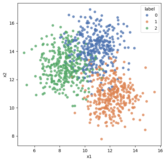
import pandas as pdimport matplotlib.pyplot as pltimport seaborn as snsfrom sklearn.datasets import make_blobsX, y, centers = make_blobs(n_samples=1000, centers=3, n_features=2, random_state=0, return_centers=True, center_box=(0,20), cluster_std =1.1)
plt.figure(figsize=(6,6))sns.scatterplot(data = df, x ='x1', y ='x2', hue ='label', alpha =.8, palette="deep",edgecolor ='None');
7.7 Exploratory Data Analysis using Python
After all of this lengthy introduction, we are finally ready to get started with actually performing some EDA.
As mentioned earlier, EDA is unstructured exploration, there is not a set of set activities you must perform. Generally, you probe the data, and depending upon what you discover, you ask more questions.
Things we will do:
Look at how to read different types of data
Understand how to access in-built datasets in Python
Calculate summary statistics covered in the prior class (refer list to the right)
Perform basic graphing using Pandas to explore the data
Understand group-by and pivoting functions (the split-apply-combine process)
Look at pandas-profiling, a library that can perform many data exploration tasks
Pandas is a library we will be using often, and is something we will use to explore data and perform EDA. We will also use NumPy and SciPy.
Code
# Load the regular librariesimport pandas as pdimport numpy as npimport seaborn as snsimport matplotlib.pyplot as plt
7.7.1 A note on managing working directories
A very basic problem one runs into when trying to load datafiles is the file path - and if the file is not located in the current working directory for Python.
Generally, reading a CSV file is simple - pd.read_csv and pointing to the filename does the trick. If the file is there but pandas returns an error, that could be because the file may not be located in your working directory. In such a case, enter the complete path to the file.
Alternatively, you can bring the file to your working directory. To check and change your working directory, use the following code:
Code
import os# To check current working directory:os.getcwd()
'C:\\Users\\user\\Google Drive\\jupyter'
Or, you could type pwd in a cell. Be aware that pwd should be on the first line of the cell!
Code
pwd
'C:\\Users\\user\\Google Drive\\jupyter'
Code
# To change working directoryos.chdir(r'C:\Users\user\Google Drive\jupyter')
7.7.2 EDA on the diamonds dataset
7.7.2.1 Questions we might like answered
Below is a repeat of what was said in the introduction to this chapter, just to avoid having to go back to check what we are trying to do. When performing EDA, we want to explore data in an unstructured way, and try to get a ‘feel’ for the data. The kinds of questions we may want to answer are:
How much data do we have - number of rows in the data?
How many columns, or fields do we have in the dataset?
Data types - which of the columns appear to be numeric, dates or strings?
Names of the columns, and do they tell us anything?
A visual review of a sample of the dataset
Completeness of the dataset, are missing values obvious? Columns that are largely empty?
Unique values for columns that appear to be categorical, and how many observations of each category?
For numeric columns, the range of values (calculated from min and max values)
Distributions for the different columns, possibly graphed
Correlations between the different columns
Code
display(Markdown('**Lab exercise - getting started with EDA**'))YouTubeVideo('kxPMkSctKmg', width=672, height=378)
Lab exercise - getting started with EDA
7.7.2.2 Load data
We will start our exploration with the diamonds dataset.
The ‘diamonds’ has 50k+ records, each representing a single diamond. The weight and other attributes are available, and so is the price.
The dataset allows us to experiment with a variety of prediction techniques and algorithms. Below are the columns in the dataset, and their description.
Column
Description
price
price in US dollars (\$326–\$18,823)
carat
weight of the diamond (0.2–5.01)
cut
quality of the cut (Fair, Good, Very Good, Premium, Ideal)
color
diamond colour, from J (worst) to D (best)
clarity
a measurement of how clear the diamond is (I1 (worst), SI2, SI1, VS2, VS1, VVS2, VVS1, IF (best))
x
length in mm (0–10.74)
y
width in mm (0–58.9)
z
depth in mm (0–31.8)
depth
total depth percentage = z / mean(x, y) = 2 * z / (x + y) (43–79)
table
width of top of diamond relative to widest point (43–95)
Code
# Load data from seaborndf = sns.load_dataset('diamonds')df
carat
cut
color
clarity
depth
table
price
x
y
z
0
0.23
Ideal
E
SI2
61.5
55.0
326
3.95
3.98
2.43
1
0.21
Premium
E
SI1
59.8
61.0
326
3.89
3.84
2.31
2
0.23
Good
E
VS1
56.9
65.0
327
4.05
4.07
2.31
3
0.29
Premium
I
VS2
62.4
58.0
334
4.20
4.23
2.63
4
0.31
Good
J
SI2
63.3
58.0
335
4.34
4.35
2.75
...
...
...
...
...
...
...
...
...
...
...
53935
0.72
Ideal
D
SI1
60.8
57.0
2757
5.75
5.76
3.50
53936
0.72
Good
D
SI1
63.1
55.0
2757
5.69
5.75
3.61
53937
0.70
Very Good
D
SI1
62.8
60.0
2757
5.66
5.68
3.56
53938
0.86
Premium
H
SI2
61.0
58.0
2757
6.15
6.12
3.74
53939
0.75
Ideal
D
SI2
62.2
55.0
2757
5.83
5.87
3.64
53940 rows × 10 columns
7.7.2.3 Descriptive stats
Pandas describe() function provides a variety of summary statistics. Review the table below. Notice the categorical variables were ignored. This is because descriptive stats do not make sense for categorical variables.
Code
# Let us look at some descriptive statistics for the numerical variablesdf.describe()
Similarly, df.shape gives you a tuple with the counts of rows and columns.
Trivia:
- Note there is no () after df.shape, as it is a property. Properties are the ‘attributes’ of the object that can be set using methods. - Methods are like functions, but are inbuilt, and apply to an object. They are part of the class definition for the object.
Exploring individual columns
Pandas provide a large number of functions that allow us to explore several statistics relating to individual variables.
Measures
Function (from Pandas, unless otherwise stated)
Central Tendency
Mean
mean()
Geometric Mean
gmean() (from scipy.stats)
Median
median()
Mode
mode()
Measures of Variability
Range
max() - min()
Variance
var()
Standard Deviation
std()
Coefficient of Variation
std() / mean()
Measures of Association
Covariance
cov()
Correlation
corr()
Analyzing Distributions
Percentiles
quantile()
Quartiles
quantile()
Z-Scores
zscore (from scipy)
We examine many of these in action below.
7.7.2.4 Functions for descriptive stats
Code
# Meandf.mean(numeric_only=True)
carat       0.797940
depth      61.749405
table      57.457184
price    3932.799722
x           5.731157
y           5.734526
z           3.538734
dtype: float64
Code
# Mediandf.median(numeric_only=True)
carat       0.70
depth      61.80
table      57.00
price    2401.00
x           5.70
y           5.71
z           3.53
dtype: float64
Code
# Modedf.mode()
carat
cut
color
clarity
depth
table
price
x
y
z
0
0.3
Ideal
G
SI1
62.0
56.0
605
4.37
4.34
2.7
Code
# Min, also max works as welldf.min(numeric_only=True)
carat      0.2
depth     43.0
table     43.0
price    326.0
x          0.0
y          0.0
z          0.0
dtype: float64
Code
# Variancedf.var(numeric_only=True)
carat    2.246867e-01
depth    2.052404e+00
table    4.992948e+00
price    1.591563e+07
x        1.258347e+00
y        1.304472e+00
z        4.980109e-01
dtype: float64
Code
# Standard Deviationdf.std(numeric_only=True)
carat       0.474011
depth       1.432621
table       2.234491
price    3989.439738
x           1.121761
y           1.142135
z           0.705699
dtype: float64
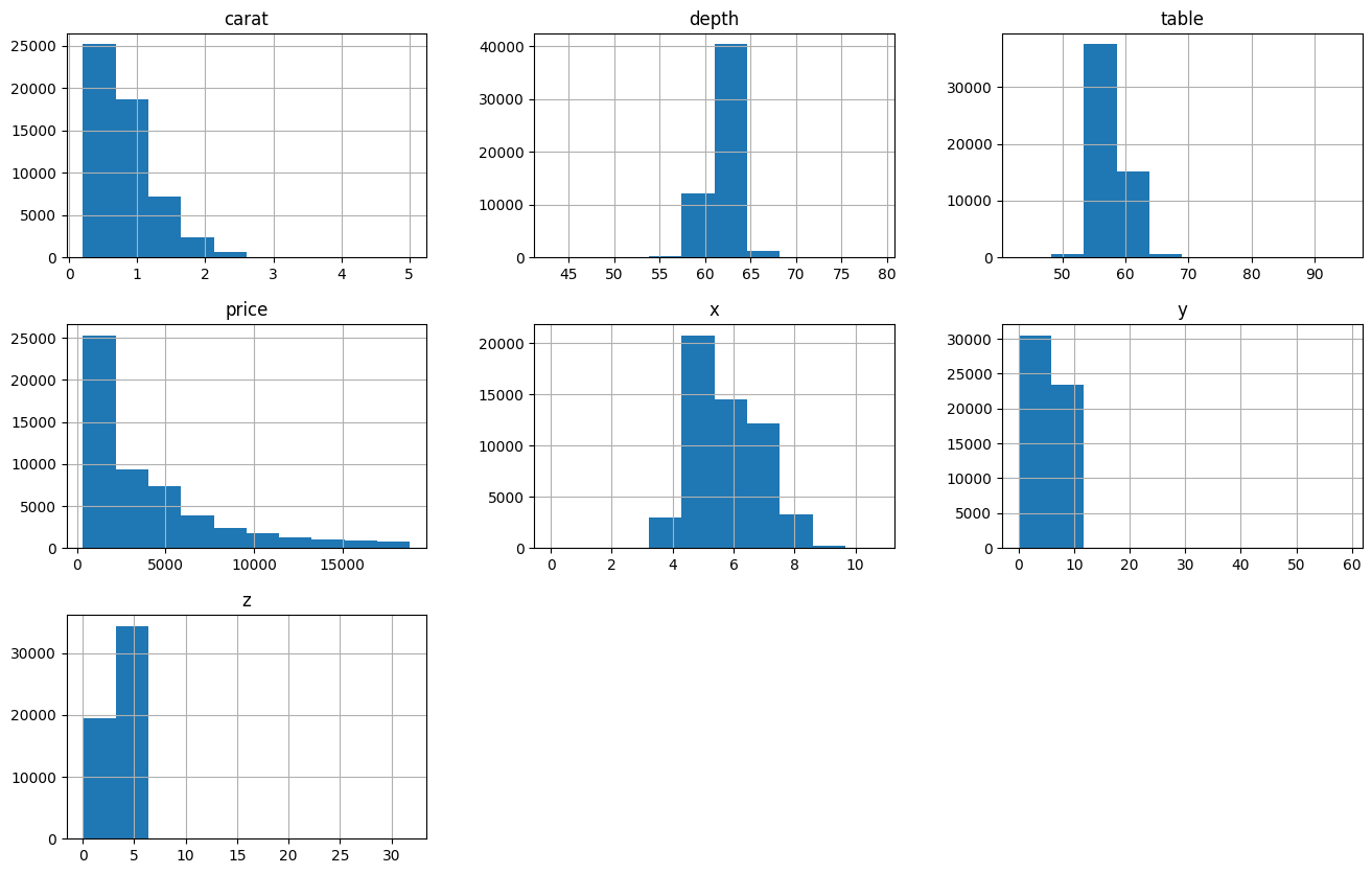
7.7.2.5 Some quick histograms
Histograms allow us to look at the distribution of the data. The df.colname.hist() function allows us to create quick histograms (or column charts in case of categorical variables).
Visualization using Matplotlib is covered in a different chapter.
Code
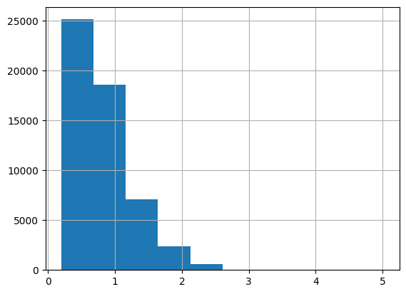
# A quick histogramdf.carat.hist();
Code
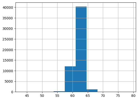
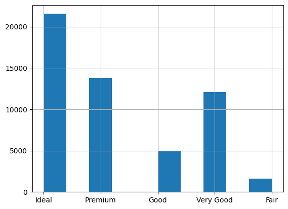
df.depth.hist();
Code
df.cut.hist();
Code
# All togetherdf.hist(figsize=(16,10));
7.7.2.6 Calculate range
Code
# Let us calculate the range manuallydf.depth.max() - df.depth.min()
36.0
7.7.2.7 Covariance and correlations
Code
# Let us do the covariance matrix, which is a one-liner with pandasdf.cov(numeric_only=True)
carat
depth
table
price
x
y
z
carat
0.224687
0.019167
0.192365
1.742765e+03
0.518484
0.515248
0.318917
depth
0.019167
2.052404
-0.946840
-6.085371e+01
-0.040641
-0.048009
0.095968
table
0.192365
-0.946840
4.992948
1.133318e+03
0.489643
0.468972
0.237996
price
1742.765364
-60.853712
1133.318064
1.591563e+07
3958.021491
3943.270810
2424.712613
x
0.518484
-0.040641
0.489643
3.958021e+03
1.258347
1.248789
0.768487
y
0.515248
-0.048009
0.468972
3.943271e+03
1.248789
1.304472
0.767320
z
0.318917
0.095968
0.237996
2.424713e+03
0.768487
0.767320
0.498011
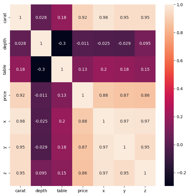
Code
# Now the correlation matrix - another one-linerdf.corr(numeric_only=True)
carat
depth
table
price
x
y
z
carat
1.000000
0.028224
0.181618
0.921591
0.975094
0.951722
0.953387
depth
0.028224
1.000000
-0.295779
-0.010647
-0.025289
-0.029341
0.094924
table
0.181618
-0.295779
1.000000
0.127134
0.195344
0.183760
0.150929
price
0.921591
-0.010647
0.127134
1.000000
0.884435
0.865421
0.861249
x
0.975094
-0.025289
0.195344
0.884435
1.000000
0.974701
0.970772
y
0.951722
-0.029341
0.183760
0.865421
0.974701
1.000000
0.952006
z
0.953387
0.094924
0.150929
0.861249
0.970772
0.952006
1.000000
Code
# We can also calculate the correlations individually between given variablesdf[['carat', 'depth']].corr(numeric_only=True)
# Z-scores for two of the columns (x - mean(x))/std(x)from scipy.stats import zscorezscores = zscore(df[['carat', 'depth']])# Verify z-scores have mean of 0 and standard deviation of 1:print('Z-scores: \n', zscores, '\n')print('Mean is: ', zscores.mean(axis =0), '\n')print('Std Deviation is: ', zscores.std(axis =0), '\n')
Sort: df.sort_values(['price', 'table'], ascending = [False, True]).head()
Unique values: df.cut.unique()
Count of unique values: df.cut.nunique()
Value Counts: df.cut.value_counts()
Take a sample from a dataframe: diamonds.sample(4) (or n=4)
Rename columns: df.rename(columns = {'price':'dollars'}, inplace = True)
7.8Split-Apply-Combine
The phrase Split-Apply-Combine was made popular by Hadley Wickham, who is the author of the popular dplyr package in R. His original paper on the topic can be downloaded at https://www.jstatsoft.org/article/download/v040i01/468
Conceptually, it involves:
- Splitting the data into sub-groups based on some filtering criteria
- Applying a function to each sub-group and obtaining a result
- Combining the results into one single dataframe.
Split-Apply-Combine does not represent three separate steps in data analysis, but a way to think about solving problems by breaking them up into manageable pieces, operate on each piece independently, and put all the pieces back together.
In Python, the Split-Apply-Combine operations are implemented using different functions such as pivot, pivot_table, crosstab, groupby and possibly others.
Ref: http://www.jstatsoft.org/v40/i01/
Code
display(Markdown('**This video provides an overview of EDA without code**'))YouTubeVideo('YW6N3JIOCM0', width=672, height=378)
This video provides an overview of EDA without code
Even though stack and unstack do not pivot data, they reshape a data in a fundamental way that deserves a reference alongside the standard split-apply-combine techniques.
What stack does is to completely flatten out a dataframe by bringing all columns down against the index. The index becomes a multi-level index, and all the columns show up against every single row.
The result is a pandas series, with as many rows as the rows times columns in the original dataset.
You can then move the index into the columns of a dataframe by doing reset_index().
Let us first consider a simpler dataframe with just a few entries.
We had 150 rows and 5 columns in our original dataset, and we would therefore expect to have 150*5 = 750 items in our stacked series. Which we can verify.
Code
iris.shape[0] * iris.shape[1]
750
Example 3:
We stack the mtcars dataset.
Code
mtcars = sm.datasets.get_rdataset('mtcars').data
Code
mtcars
mpg
cyl
disp
hp
drat
wt
qsec
vs
am
gear
carb
rownames
Mazda RX4
21.0
6
160.0
110
3.90
2.620
16.46
0
1
4
4
Mazda RX4 Wag
21.0
6
160.0
110
3.90
2.875
17.02
0
1
4
4
Datsun 710
22.8
4
108.0
93
3.85
2.320
18.61
1
1
4
1
Hornet 4 Drive
21.4
6
258.0
110
3.08
3.215
19.44
1
0
3
1
Hornet Sportabout
18.7
8
360.0
175
3.15
3.440
17.02
0
0
3
2
Valiant
18.1
6
225.0
105
2.76
3.460
20.22
1
0
3
1
Duster 360
14.3
8
360.0
245
3.21
3.570
15.84
0
0
3
4
Merc 240D
24.4
4
146.7
62
3.69
3.190
20.00
1
0
4
2
Merc 230
22.8
4
140.8
95
3.92
3.150
22.90
1
0
4
2
Merc 280
19.2
6
167.6
123
3.92
3.440
18.30
1
0
4
4
Merc 280C
17.8
6
167.6
123
3.92
3.440
18.90
1
0
4
4
Merc 450SE
16.4
8
275.8
180
3.07
4.070
17.40
0
0
3
3
Merc 450SL
17.3
8
275.8
180
3.07
3.730
17.60
0
0
3
3
Merc 450SLC
15.2
8
275.8
180
3.07
3.780
18.00
0
0
3
3
Cadillac Fleetwood
10.4
8
472.0
205
2.93
5.250
17.98
0
0
3
4
Lincoln Continental
10.4
8
460.0
215
3.00
5.424
17.82
0
0
3
4
Chrysler Imperial
14.7
8
440.0
230
3.23
5.345
17.42
0
0
3
4
Fiat 128
32.4
4
78.7
66
4.08
2.200
19.47
1
1
4
1
Honda Civic
30.4
4
75.7
52
4.93
1.615
18.52
1
1
4
2
Toyota Corolla
33.9
4
71.1
65
4.22
1.835
19.90
1
1
4
1
Toyota Corona
21.5
4
120.1
97
3.70
2.465
20.01
1
0
3
1
Dodge Challenger
15.5
8
318.0
150
2.76
3.520
16.87
0
0
3
2
AMC Javelin
15.2
8
304.0
150
3.15
3.435
17.30
0
0
3
2
Camaro Z28
13.3
8
350.0
245
3.73
3.840
15.41
0
0
3
4
Pontiac Firebird
19.2
8
400.0
175
3.08
3.845
17.05
0
0
3
2
Fiat X1-9
27.3
4
79.0
66
4.08
1.935
18.90
1
1
4
1
Porsche 914-2
26.0
4
120.3
91
4.43
2.140
16.70
0
1
5
2
Lotus Europa
30.4
4
95.1
113
3.77
1.513
16.90
1
1
5
2
Ford Pantera L
15.8
8
351.0
264
4.22
3.170
14.50
0
1
5
4
Ferrari Dino
19.7
6
145.0
175
3.62
2.770
15.50
0
1
5
6
Maserati Bora
15.0
8
301.0
335
3.54
3.570
14.60
0
1
5
8
Volvo 142E
21.4
4
121.0
109
4.11
2.780
18.60
1
1
4
2
Code
mtcars.stack()
rownames
Mazda RX4   mpg      21.0
            cyl       6.0
            disp    160.0
            hp      110.0
            drat      3.9
                    ...
Volvo 142E  qsec     18.6
            vs        1.0
            am        1.0
            gear      4.0
            carb      2.0
Length: 352, dtype: float64
7.8.2 Unstack
Unstack is the same as the stack of the transpose of a dataframe.
So you flip the rows and columns of a database, and you then do a stack.
Code
mtcars.transpose()
rownames
Mazda RX4
Mazda RX4 Wag
Datsun 710
Hornet 4 Drive
Hornet Sportabout
Valiant
Duster 360
Merc 240D
Merc 230
Merc 280
...
AMC Javelin
Camaro Z28
Pontiac Firebird
Fiat X1-9
Porsche 914-2
Lotus Europa
Ford Pantera L
Ferrari Dino
Maserati Bora
Volvo 142E
mpg
21.00
21.000
22.80
21.400
18.70
18.10
14.30
24.40
22.80
19.20
...
15.200
13.30
19.200
27.300
26.00
30.400
15.80
19.70
15.00
21.40
cyl
6.00
6.000
4.00
6.000
8.00
6.00
8.00
4.00
4.00
6.00
...
8.000
8.00
8.000
4.000
4.00
4.000
8.00
6.00
8.00
4.00
disp
160.00
160.000
108.00
258.000
360.00
225.00
360.00
146.70
140.80
167.60
...
304.000
350.00
400.000
79.000
120.30
95.100
351.00
145.00
301.00
121.00
hp
110.00
110.000
93.00
110.000
175.00
105.00
245.00
62.00
95.00
123.00
...
150.000
245.00
175.000
66.000
91.00
113.000
264.00
175.00
335.00
109.00
drat
3.90
3.900
3.85
3.080
3.15
2.76
3.21
3.69
3.92
3.92
...
3.150
3.73
3.080
4.080
4.43
3.770
4.22
3.62
3.54
4.11
wt
2.62
2.875
2.32
3.215
3.44
3.46
3.57
3.19
3.15
3.44
...
3.435
3.84
3.845
1.935
2.14
1.513
3.17
2.77
3.57
2.78
qsec
16.46
17.020
18.61
19.440
17.02
20.22
15.84
20.00
22.90
18.30
...
17.300
15.41
17.050
18.900
16.70
16.900
14.50
15.50
14.60
18.60
vs
0.00
0.000
1.00
1.000
0.00
1.00
0.00
1.00
1.00
1.00
...
0.000
0.00
0.000
1.000
0.00
1.000
0.00
0.00
0.00
1.00
am
1.00
1.000
1.00
0.000
0.00
0.00
0.00
0.00
0.00
0.00
...
0.000
0.00
0.000
1.000
1.00
1.000
1.00
1.00
1.00
1.00
gear
4.00
4.000
4.00
3.000
3.00
3.00
3.00
4.00
4.00
4.00
...
3.000
3.00
3.000
4.000
5.00
5.000
5.00
5.00
5.00
4.00
carb
4.00
4.000
1.00
1.000
2.00
1.00
4.00
2.00
2.00
4.00
...
2.000
4.00
2.000
1.000
2.00
2.000
4.00
6.00
8.00
2.00
11 rows × 32 columns
Code
mtcars.unstack()
      rownames
mpg   Mazda RX4            21.0
      Mazda RX4 Wag        21.0
      Datsun 710           22.8
      Hornet 4 Drive       21.4
      Hornet Sportabout    18.7
                           ...
carb  Lotus Europa          2.0
      Ford Pantera L        4.0
      Ferrari Dino          6.0
      Maserati Bora         8.0
      Volvo 142E            2.0
Length: 352, dtype: float64
Code
mtcars.transpose().stack()
      rownames
mpg   Mazda RX4            21.0
      Mazda RX4 Wag        21.0
      Datsun 710           22.8
      Hornet 4 Drive       21.4
      Hornet Sportabout    18.7
                           ...
carb  Lotus Europa          2.0
      Ford Pantera L        4.0
      Ferrari Dino          6.0
      Maserati Bora         8.0
      Volvo 142E            2.0
Length: 352, dtype: float64
Code
# Check the row countmtcars.stack().shape
(352,)
Code
# Expected row count in stackmtcars.shape[0] * mtcars.shape[1]
352
7.8.3 Pivot table
A powerful way the idea behind split-apply_combine is implemented is through pivot tables. Pivot tables allow reshaping the data into useful summaries. Pivot tables are widely used by Excel users, and you will find them used in reports, presentations and analysis of all types. Pandas offers a great deal of flexibility for creating pivot tables using the pivot_table function.
The pivot_table function is essentially a copy of the Excel functionality.
index - On the left is the index, and you can specify multiple columns there. Each unique value in that index column will have a separate line. Under each of these lines, there will be a line for each value of the second column in the index, and so on.
columns - On the top are the columns, again in the order in which specified in the parameters to the function. The first column specified is on the top, and underneath will be all unique values of that column. This is followed by the next column in the list, and so on.
values - Inside the table itself are values derived from the columns named in the values parameter. The default for values is the mean of the value columns, but you can change it to other functions using aggfunc.
aggfunc - Next is aggfunc. You can specify any function from any library that returns a single value.
CAUTION
It is really easy to get pivot tables wrong and get something incomprehensible. To create a sensible pivot table, it makes sense to: - have categorical columns in both index and columns. If you use numerical variables in either, the length of your columns/rows will explode unless the number of unique values is limited.
- have columns in the values parameter that lend themselves to the aggregation function specified. So if you specify a categorical column for values, and ask pandas to show the mean, you will be setting yourself up for disappointment. If you are using a categorical column for values, be sure to use an appropriate aggregation function eg count.
Code
mtcars.head()
mpg
cyl
disp
hp
drat
wt
qsec
vs
am
gear
carb
rownames
Mazda RX4
21.0
6
160.0
110
3.90
2.620
16.46
0
1
4
4
Mazda RX4 Wag
21.0
6
160.0
110
3.90
2.875
17.02
0
1
4
4
Datsun 710
22.8
4
108.0
93
3.85
2.320
18.61
1
1
4
1
Hornet 4 Drive
21.4
6
258.0
110
3.08
3.215
19.44
1
0
3
1
Hornet Sportabout
18.7
8
360.0
175
3.15
3.440
17.02
0
0
3
2
Code
# Some transformations to help understand pivots bettermtcars.cyl = mtcars.cyl.replace({4: 'Four', 6: 'Six', 8: 'Eight'} )mtcars.am = mtcars.am.replace({1: 'Automatic', 0: 'Manual'} )
C:\Users\user\AppData\Local\Temp\ipykernel_13000\3088381430.py:3: FutureWarning: The default value of observed=False is deprecated and will change to observed=True in a future version of pandas. Specify observed=False to silence this warning and retain the current behavior
  diamonds.pivot_table(index = ['clarity', 'cut'],
C:\Users\user\AppData\Local\Temp\ipykernel_13000\3088381430.py:3: FutureWarning: The provided callable <function mean at 0x000001D76EDF1C60> is currently using SeriesGroupBy.mean. In a future version of pandas, the provided callable will be used directly. To keep current behavior pass the string "mean" instead.
  diamonds.pivot_table(index = ['clarity', 'cut'],
C:\Users\user\AppData\Local\Temp\ipykernel_13000\3088381430.py:3: FutureWarning: The provided callable <built-in function min> is currently using SeriesGroupBy.min. In a future version of pandas, the provided callable will be used directly. To keep current behavior pass the string "min" instead.
  diamonds.pivot_table(index = ['clarity', 'cut'],
C:\Users\user\AppData\Local\Temp\ipykernel_13000\3088381430.py:3: FutureWarning: The provided callable <built-in function max> is currently using SeriesGroupBy.max. In a future version of pandas, the provided callable will be used directly. To keep current behavior pass the string "max" instead.
  diamonds.pivot_table(index = ['clarity', 'cut'],
C:\Users\user\AppData\Local\Temp\ipykernel_13000\3088381430.py:3: FutureWarning: The provided callable <function median at 0x000001D76EF56520> is currently using SeriesGroupBy.median. In a future version of pandas, the provided callable will be used directly. To keep current behavior pass the string "median" instead.
  diamonds.pivot_table(index = ['clarity', 'cut'],
depth
price
x
mean
max
...
min
median
color
D
E
F
G
H
I
J
D
E
F
...
H
I
J
D
E
F
G
H
I
J
clarity
cut
IF
Ideal
61.496429
61.716456
61.614925
61.663951
61.557522
61.751579
61.956000
17590.0
18700.0
18435.0
...
468.0
587.0
489.0
5.315
4.430
4.400
4.510
4.610
4.570
4.710
Premium
61.070000
60.859259
61.112903
60.904598
61.290000
61.078261
61.458333
18279.0
17663.0
18102.0
...
739.0
631.0
533.0
6.100
4.640
4.390
4.640
4.440
4.830
6.570
Very Good
61.513043
61.160465
61.123881
61.470886
61.858621
61.278947
61.387500
18542.0
12895.0
18552.0
...
369.0
673.0
529.0
6.170
4.770
4.730
4.800
4.710
5.490
4.715
Good
60.877778
61.811111
60.620000
61.509091
61.975000
62.150000
62.466667
17499.0
6804.0
9867.0
...
1440.0
631.0
827.0
6.260
4.280
5.120
5.025
6.080
4.755
5.025
Fair
60.766667
NaN
58.925000
61.300000
NaN
NaN
NaN
2211.0
NaN
3205.0
...
NaN
NaN
NaN
4.680
NaN
5.285
4.905
NaN
NaN
NaN
VVS1
Ideal
61.710417
61.608358
61.649545
61.667508
61.720552
61.794972
61.844828
16253.0
16256.0
18682.0
...
449.0
414.0
461.0
4.730
4.490
4.670
4.760
4.765
4.880
4.890
Premium
61.182500
61.219048
61.121250
61.060234
61.353571
61.627381
61.754167
17496.0
14952.0
14196.0
...
432.0
414.0
775.0
4.775
4.510
4.825
4.740
4.430
4.800
7.145
Very Good
61.675000
61.504118
61.545977
61.586316
61.980000
62.165217
61.684211
17932.0
15878.0
18777.0
...
434.0
336.0
544.0
4.685
4.240
4.505
4.620
4.690
4.910
5.700
Good
61.653846
61.525581
62.291429
61.987805
62.477419
62.990909
63.500000
8239.0
10696.0
11182.0
...
401.0
552.0
4633.0
4.680
4.450
4.470
4.860
4.430
5.295
6.290
Fair
61.666667
59.600000
59.100000
60.066667
56.500000
63.500000
67.600000
10752.0
8529.0
12648.0
...
4115.0
4194.0
1691.0
4.920
5.340
4.850
5.670
6.380
5.980
5.560
VVS2
Ideal
61.584859
61.681460
61.646923
61.692377
61.753633
61.883708
61.759259
16130.0
18188.0
18614.0
...
442.0
412.0
413.0
4.770
4.710
5.120
5.180
4.670
5.110
5.760
Premium
61.024468
61.076860
61.277397
61.297091
61.496610
61.446341
61.435294
17216.0
17667.0
17203.0
...
486.0
526.0
778.0
4.860
4.680
5.165
5.150
4.570
4.750
7.115
Very Good
61.328369
61.497315
61.541767
61.821523
61.895862
61.957746
62.410345
17545.0
17689.0
17317.0
...
378.0
427.0
336.0
4.570
4.280
4.830
5.100
4.670
5.600
6.860
Good
62.284000
62.192308
61.824000
62.625333
62.562222
62.500000
61.661538
8943.0
17449.0
14654.0
...
440.0
579.0
375.0
4.740
4.895
5.300
5.060
5.220
5.625
6.340
Fair
61.677778
60.623077
62.610000
64.376471
63.600000
63.400000
66.000000
10562.0
7918.0
16364.0
...
922.0
1401.0
2998.0
4.950
5.270
5.200
5.430
6.030
5.780
6.290
VS1
Ideal
61.620228
61.638449
61.660065
61.696642
61.789293
61.813971
61.835323
17659.0
18729.0
18780.0
...
423.0
358.0
340.0
4.880
4.770
5.280
5.310
5.230
5.750
6.150
Premium
61.132824
61.119863
61.197241
61.419965
61.398512
61.297285
61.565359
17936.0
17552.0
18598.0
...
382.0
355.0
394.0
5.630
5.135
5.730
5.270
5.695
6.500
6.880
Very Good
61.553143
61.593174
61.495222
61.701620
62.004669
61.947805
62.024167
16750.0
16988.0
17685.0
...
338.0
397.0
394.0
5.120
5.200
5.560
5.295
5.750
6.120
6.175
Good
61.597674
61.602247
61.317424
62.446711
62.277922
62.369903
62.528846
17111.0
17400.0
17330.0
...
435.0
457.0
394.0
5.610
5.670
5.330
5.915
5.670
6.060
5.705
Fair
63.160000
61.371429
62.430303
63.353333
63.309375
62.796000
63.675000
7083.0
15584.0
17995.0
...
1134.0
735.0
949.0
5.560
5.435
5.940
5.620
6.100
6.000
6.210
VS2
Ideal
61.688478
61.717077
61.726394
61.726813
61.804317
61.778082
61.734914
18318.0
17825.0
18421.0
...
367.0
371.0
384.0
4.815
5.090
5.170
5.655
5.690
5.920
6.480
Premium
61.146313
61.259459
61.303231
61.287933
61.324624
61.296825
61.381683
16921.0
18342.0
18791.0
...
471.0
334.0
368.0
5.120
5.170
5.390
5.860
6.495
6.920
6.900
Very Good
61.968285
61.782903
61.807082
61.901670
61.913564
61.715693
61.868478
17153.0
18557.0
18430.0
...
376.0
379.0
357.0
5.160
5.300
5.640
5.870
6.125
6.285
6.560
Good
62.758654
61.877500
62.487500
62.365104
62.675362
62.107273
62.346667
17760.0
15385.0
17597.0
...
470.0
435.0
368.0
5.560
5.685
5.685
6.015
6.025
6.310
6.525
Fair
62.684000
64.476190
63.577358
63.880000
63.960976
62.384375
63.973913
15152.0
12829.0
13853.0
...
704.0
855.0
416.0
6.040
5.430
5.820
6.080
6.090
6.045
6.080
SI1
Ideal
61.736179
61.713708
61.669079
61.717424
61.763041
61.791468
61.849794
16575.0
18193.0
18306.0
...
357.0
382.0
367.0
5.160
5.375
5.730
5.720
6.420
6.470
6.640
Premium
61.254317
61.229153
61.346875
61.340106
61.332824
61.318256
61.306699
17776.0
16957.0
18735.0
...
421.0
394.0
363.0
5.300
5.680
5.940
6.160
6.580
6.780
6.880
Very Good
61.822470
61.947764
61.942039
61.963502
61.990676
62.075978
61.873626
16286.0
18731.0
18759.0
...
337.0
382.0
351.0
5.650
5.660
5.780
5.695
6.350
6.425
6.460
Good
62.755696
62.754085
62.499267
62.896618
62.585957
62.825455
62.496591
18468.0
18027.0
18376.0
...
402.0
377.0
339.0
5.590
5.600
5.750
6.070
6.180
6.230
6.430
Fair
64.634483
63.226154
63.230120
64.513043
64.488000
63.883333
63.010714
16386.0
15330.0
16280.0
...
659.0
1697.0
497.0
6.080
6.060
6.060
6.070
6.260
6.365
6.535
SI2
Ideal
61.673876
61.680171
61.708830
61.732510
61.627111
61.751095
61.883636
18693.0
18128.0
18578.0
...
362.0
348.0
344.0
5.730
6.100
6.130
6.330
6.600
6.920
6.835
Premium
61.099287
61.095376
61.174761
61.183943
61.219194
61.305128
61.280745
18575.0
18477.0
18784.0
...
368.0
500.0
405.0
6.320
6.340
6.420
6.550
6.810
7.000
7.360
Very Good
61.743631
61.764719
61.782216
62.011009
62.006997
61.935500
61.835938
18526.0
18128.0
18692.0
...
393.0
383.0
430.0
6.290
6.180
6.270
6.330
6.620
6.790
6.795
Good
62.063229
61.986634
62.250746
62.544172
62.391139
62.365432
62.388679
17094.0
18236.0
18686.0
...
368.0
351.0
335.0
6.110
6.040
6.320
6.320
6.410
6.910
6.750
Fair
64.703571
63.448718
63.834831
64.573750
64.931868
65.564444
64.511111
16086.0
15540.0
17405.0
...
1059.0
1625.0
1362.0
6.130
6.280
6.260
6.325
6.650
7.050
6.560
I1
Ideal
61.453846
61.850000
61.588095
61.400000
61.657895
61.729412
63.500000
13156.0
9072.0
10685.0
...
3080.0
2239.0
2370.0
6.730
6.510
6.560
6.765
6.925
6.820
7.665
Premium
61.900000
60.806667
61.150000
61.113043
61.247826
61.291667
61.300000
6300.0
10453.0
9967.0
...
452.0
1107.0
945.0
6.645
6.525
6.465
6.645
6.620
7.100
6.900
Very Good
62.200000
61.481818
61.561538
61.943750
61.816667
62.100000
61.737500
3816.0
10340.0
9789.0
...
2850.0
1235.0
2048.0
6.180
6.500
6.740
6.430
7.290
7.050
7.060
Good
61.350000
61.660870
62.889474
62.568421
61.757143
61.622222
61.650000
6088.0
11548.0
6686.0
...
1134.0
1111.0
1945.0
6.720
7.010
6.090
6.640
6.400
6.930
6.950
Fair
65.600000
65.644444
65.657143
65.333962
65.759615
65.729412
66.460870
15964.0
3692.0
7294.0
...
1058.0
1014.0
1066.0
7.325
6.180
5.640
6.170
6.930
6.660
7.430
40 rows × 35 columns
Code
# Let us create a dataframe with random variablesnp.random.seed(1)n =2500df = pd.DataFrame( {'state': list(np.random.choice(["New York", "Florida", "California"], size=(n))), 'gender': list(np.random.choice(["Male", "Female"], size=(n), p=[.4, .6])),'education': list(np.random.choice(["High School", "Undergrad", "Grad"], size=(n))),'housing': list(np.random.choice(["Rent", "Own"], size=(n))), 'height': list(np.random.randint(140,200,n)),'weight': list(np.random.randint(100,150,n)),'income': list(np.random.randint(50,250,n)),'computers': list(np.random.randint(0,6,n)) })
C:\Users\user\AppData\Local\Temp\ipykernel_13000\4063274067.py:1: FutureWarning: The provided callable <function median at 0x000001D76EF56520> is currently using SeriesGroupBy.median. In a future version of pandas, the provided callable will be used directly. To keep current behavior pass the string "median" instead.
df.pivot_table(index = ['state'],
computers
gender
mean
median
len
education
Grad
High School
Undergrad
Grad
High School
Undergrad
Grad
High School
Undergrad
housing
Own
Rent
Own
Rent
Own
Rent
Own
Rent
Own
Rent
Own
Rent
Own
Rent
Own
Rent
Own
Rent
state
California
2.659574
2.527778
2.550000
2.446667
2.335484
2.634615
3.0
3.0
3.0
2.0
2.0
3.0
141
144
120
150
155
156
Florida
2.344538
2.647059
2.414815
2.365672
2.674242
2.246377
2.0
3.0
2.0
2.0
3.0
2.0
119
136
135
134
132
138
New York
2.524194
2.317073
2.291667
2.564885
2.520270
2.505882
3.0
2.0
2.0
3.0
3.0
2.0
124
123
144
131
148
170
7.8.4 Pivot
Pivot is a simpler version of pivot_table. It cannot do any aggregation function, it just shows the values of the ‘value’ columns at the intersection of the ‘index’ and the ‘columns’.
There are three parameters for pivot: 1. index - which columns in the dataframe should be the index. This is optional. If not specified, it uses the index of the dataframe.
2. columns - which dataframe columns should appear on the top as columns in the result. For each entry in the column parameter, it will create a separate column for each unique value of that column. So if ‘carb’ can be 1, 2 or 4, it will show 1, 2 and 4 on the top. 3. values - which column’s values to show at the intersection of index and columns. If there is more than one value (even if the multiple values are identical), pivot will throw an error. (for example, in mtcars_small, if yuou put cyl 4,6,8 on the left as index, and am 0,1 on the top as columns, and mpg as values, you have two cars at their intersection.)
Pivot can be better than pivot_table as it brings in the value at the intersection of index and columns as-is, which is what you need sometimes without having to add, mean, or count them.
# We consider only the first 3 rows of this new dataframe.# Look how in the values we have a categorical variable.df.iloc[:3].pivot(index ='weight', columns ='height', values ='animal')
height
1
3
7
weight
0
cat
NaN
NaN
2
NaN
dog
NaN
6
NaN
NaN
cow
7.8.5 Crosstab
Cross computes a frequency table given an index and columns of categorical variables (as a data frame column, series, or numpy array). However it is possible to specify an aggfunc as well, that makes it like a pivot_table.
You can pass normalize = True, or index, or columns, and it will normalize based on totals, or by the rows or by the columns.
Code
df = sns.load_dataset('diamonds')df
carat
cut
color
clarity
depth
table
price
x
y
z
0
0.23
Ideal
E
SI2
61.5
55.0
326
3.95
3.98
2.43
1
0.21
Premium
E
SI1
59.8
61.0
326
3.89
3.84
2.31
2
0.23
Good
E
VS1
56.9
65.0
327
4.05
4.07
2.31
3
0.29
Premium
I
VS2
62.4
58.0
334
4.20
4.23
2.63
4
0.31
Good
J
SI2
63.3
58.0
335
4.34
4.35
2.75
...
...
...
...
...
...
...
...
...
...
...
53935
0.72
Ideal
D
SI1
60.8
57.0
2757
5.75
5.76
3.50
53936
0.72
Good
D
SI1
63.1
55.0
2757
5.69
5.75
3.61
53937
0.70
Very Good
D
SI1
62.8
60.0
2757
5.66
5.68
3.56
53938
0.86
Premium
H
SI2
61.0
58.0
2757
6.15
6.12
3.74
53939
0.75
Ideal
D
SI2
62.2
55.0
2757
5.83
5.87
3.64
53940 rows × 10 columns
Code
# Basicpd.crosstab(df.cut, df.color)
color
D
E
F
G
H
I
J
cut
Ideal
2834
3903
3826
4884
3115
2093
896
Premium
1603
2337
2331
2924
2360
1428
808
Very Good
1513
2400
2164
2299
1824
1204
678
Good
662
933
909
871
702
522
307
Fair
163
224
312
314
303
175
119
Code
# With marginspd.crosstab(df.cut, df.color, margins =True)
color
D
E
F
G
H
I
J
All
cut
Ideal
2834
3903
3826
4884
3115
2093
896
21551
Premium
1603
2337
2331
2924
2360
1428
808
13791
Very Good
1513
2400
2164
2299
1824
1204
678
12082
Good
662
933
909
871
702
522
307
4906
Fair
163
224
312
314
303
175
119
1610
All
6775
9797
9542
11292
8304
5422
2808
53940
Code
# With margins and normalizedpd.crosstab(df.cut, df.color, margins =True, normalize =True)
color
D
E
F
G
H
I
J
All
cut
Ideal
0.052540
0.072358
0.070931
0.090545
0.057749
0.038802
0.016611
0.399537
Premium
0.029718
0.043326
0.043215
0.054208
0.043752
0.026474
0.014980
0.255673
Very Good
0.028050
0.044494
0.040119
0.042621
0.033815
0.022321
0.012570
0.223990
Good
0.012273
0.017297
0.016852
0.016148
0.013014
0.009677
0.005692
0.090953
Fair
0.003022
0.004153
0.005784
0.005821
0.005617
0.003244
0.002206
0.029848
All
0.125603
0.181628
0.176900
0.209344
0.153949
0.100519
0.052058
1.000000
Code
# Normalized by index. Rows total to 1. See how the total column 'All' has # disappeared from rows. But it has remained for the columnspd.crosstab(df.cut, df.color, margins =True, normalize ='index')
color
D
E
F
G
H
I
J
cut
Ideal
0.131502
0.181105
0.177532
0.226625
0.144541
0.097118
0.041576
Premium
0.116235
0.169458
0.169023
0.212022
0.171126
0.103546
0.058589
Very Good
0.125228
0.198643
0.179109
0.190283
0.150968
0.099652
0.056117
Good
0.134937
0.190175
0.185283
0.177538
0.143090
0.106400
0.062576
Fair
0.101242
0.139130
0.193789
0.195031
0.188199
0.108696
0.073913
All
0.125603
0.181628
0.176900
0.209344
0.153949
0.100519
0.052058
Code
# Normalized by columnspd.crosstab(df.cut, df.color, margins =True, normalize ='columns')
color
D
E
F
G
H
I
J
All
cut
Ideal
0.418303
0.398387
0.400964
0.432519
0.375120
0.386020
0.319088
0.399537
Premium
0.236605
0.238542
0.244288
0.258944
0.284200
0.263371
0.287749
0.255673
Very Good
0.223321
0.244973
0.226787
0.203595
0.219653
0.222058
0.241453
0.223990
Good
0.097712
0.095233
0.095263
0.077134
0.084538
0.096274
0.109330
0.090953
Fair
0.024059
0.022864
0.032698
0.027807
0.036488
0.032276
0.042379
0.029848
Code
# You can also pass multiple series for both the index and columnspd.crosstab([df.cut, df.color], [df.clarity])
clarity
IF
VVS1
VVS2
VS1
VS2
SI1
SI2
I1
cut
color
Ideal
D
28
144
284
351
920
738
356
13
E
79
335
507
593
1136
766
469
18
F
268
440
520
616
879
608
453
42
G
491
594
774
953
910
660
486
16
H
226
326
289
467
556
763
450
38
I
95
179
178
408
438
504
274
17
J
25
29
54
201
232
243
110
2
Premium
D
10
40
94
131
339
556
421
12
E
27
105
121
292
629
614
519
30
F
31
80
146
290
619
608
523
34
G
87
171
275
566
721
566
492
46
H
40
112
118
336
532
655
521
46
I
23
84
82
221
315
367
312
24
J
12
24
34
153
202
209
161
13
Very Good
D
23
52
141
175
309
494
314
5
E
43
170
298
293
503
626
445
22
F
67
174
249
293
466
559
343
13
G
79
190
302
432
479
474
327
16
H
29
115
145
257
376
547
343
12
I
19
69
71
205
274
358
200
8
J
8
19
29
120
184
182
128
8
Good
D
9
13
25
43
104
237
223
8
E
9
43
52
89
160
355
202
23
F
15
35
50
132
184
273
201
19
G
22
41
75
152
192
207
163
19
H
4
31
45
77
138
235
158
14
I
6
22
26
103
110
165
81
9
J
6
1
13
52
90
88
53
4
Fair
D
3
3
9
5
25
58
56
4
E
0
3
13
14
42
65
78
9
F
4
5
10
33
53
83
89
35
G
2
3
17
45
45
69
80
53
H
0
1
11
32
41
75
91
52
I
0
1
8
25
32
30
45
34
J
0
1
1
16
23
28
27
23
7.8.6 Melt
Melt is similar to Stack() but unlike stack it returns a dataframe, not a series with a multi-level index. A huge advantage is that unlike stack, you can freeze some of the columbns and stack the rest.
In melt, you specify id_vars (index variables) - these are the columns that stay untouched, and then the value_vars, that get stacked. If value_vars are not specified, all columns other than id_vars get stacked.
Opposite of melt is pivot. Pivot applies no aggfunc, just lists the values at the intersection of categorical vars it picks up from a melted dataset.
Code
# Let us create a dataframe with random variablesnp.random.seed(1)n =10df = pd.DataFrame( {'state': list(np.random.choice(["New York", "Florida", "California"], size=(n))), 'gender': list(np.random.choice(["Male", "Female"], size=(n), p=[.4, .6])),'education': list(np.random.choice(["High School", "Undergrad", "Grad"], size=(n))),'housing': list(np.random.choice(["Rent", "Own"], size=(n))), 'height': list(np.random.randint(140,200,n)),'weight': list(np.random.randint(100,150,n)),'income': list(np.random.randint(50,250,n)),'computers': list(np.random.randint(0,6,n)) })
Code
df
state
gender
education
housing
height
weight
income
computers
0
Florida
Female
Undergrad
Own
197
104
65
1
1
New York
Female
Grad
Rent
148
124
114
3
2
New York
Female
High School
Rent
170
149
246
5
3
Florida
Male
Grad
Own
147
143
75
4
4
Florida
Female
Undergrad
Rent
143
112
161
3
5
New York
Female
Undergrad
Rent
146
126
185
5
6
New York
Male
Undergrad
Own
161
116
76
1
7
Florida
Female
Undergrad
Own
189
145
203
3
8
New York
Female
Grad
Own
197
141
154
0
9
Florida
Female
Undergrad
Rent
143
118
72
0
Code
# Just to demonstrate, melt-ing the first five rows of the dfdf.head().melt(id_vars = ['state', 'gender'], value_vars = ['computers', 'income'])
state
gender
variable
value
0
Florida
Female
computers
1
1
New York
Female
computers
3
2
New York
Female
computers
5
3
Florida
Male
computers
4
4
Florida
Female
computers
3
5
Florida
Female
income
65
6
New York
Female
income
114
7
New York
Female
income
246
8
Florida
Male
income
75
9
Florida
Female
income
161
7.8.7 Groupby
Groupby returns a groupby object, to which other agg functions can be applied.
Groupby does the ‘split’ part in the split-apply-combine framework.
You do the ‘apply’ using an aggregation function against the groupby object.
‘Combine’ doesn’t need to be done separately as it is done automatically after the aggregation function is applied.
# Aggregation is done only for the columns for which an aggregation function is specifieddf.groupby(['state', 'gender']).agg({"height": "mean", "weight": "sum", "housing": "count"})
[(('Florida', 'Female'),
state gender education housing height weight income computers
0 Florida Female Undergrad Own 197 104 65 1
4 Florida Female Undergrad Rent 143 112 161 3
7 Florida Female Undergrad Own 189 145 203 3
9 Florida Female Undergrad Rent 143 118 72 0),
(('Florida', 'Male'),
state gender education housing height weight income computers
3 Florida Male Grad Own 147 143 75 4),
(('New York', 'Female'),
state gender education housing height weight income computers
1 New York Female Grad Rent 148 124 114 3
2 New York Female High School Rent 170 149 246 5
5 New York Female Undergrad Rent 146 126 185 5
8 New York Female Grad Own 197 141 154 0),
(('New York', 'Male'),
state gender education housing height weight income computers
6 New York Male Undergrad Own 161 116 76 1)]
Code
list(group)[0][1]
state
gender
education
housing
height
weight
income
computers
0
Florida
Female
Undergrad
Own
197
104
65
1
4
Florida
Female
Undergrad
Rent
143
112
161
3
7
Florida
Female
Undergrad
Own
189
145
203
3
9
Florida
Female
Undergrad
Rent
143
118
72
0
Code
type(group)
pandas.core.groupby.generic.DataFrameGroupBy
Code
# Look at groups in a groupby - more elegant version:for group_name, combined in group:print(group_name)print(combined)print('\n')
('Florida', 'Female')
state gender education housing height weight income computers
0 Florida Female Undergrad Own 197 104 65 1
4 Florida Female Undergrad Rent 143 112 161 3
7 Florida Female Undergrad Own 189 145 203 3
9 Florida Female Undergrad Rent 143 118 72 0
('Florida', 'Male')
state gender education housing height weight income computers
3 Florida Male Grad Own 147 143 75 4
('New York', 'Female')
state gender education housing height weight income computers
1 New York Female Grad Rent 148 124 114 3
2 New York Female High School Rent 170 149 246 5
5 New York Female Undergrad Rent 146 126 185 5
8 New York Female Grad Own 197 141 154 0
('New York', 'Male')
state gender education housing height weight income computers
6 New York Male Undergrad Own 161 116 76 1
Code
# How to look at a specific group - the group categorical values have to be entered as a tuplegroup.get_group(('New York', 'Male'))
state
gender
education
housing
height
weight
income
computers
6
New York
Male
Undergrad
Own
161
116
76
1
Code
# get the first row of each groupgroup.first()
education
housing
height
weight
income
computers
state
gender
Florida
Female
Undergrad
Own
197
104
65
1
Male
Grad
Own
147
143
75
4
New York
Female
Grad
Rent
148
124
114
3
Male
Undergrad
Own
161
116
76
1
Code
# Get the first record of each group.# For this to be useful, sort the original df by the right columns before groupby.group.head(1)
state
gender
education
housing
height
weight
income
computers
0
Florida
Female
Undergrad
Own
197
104
65
1
1
New York
Female
Grad
Rent
148
124
114
3
3
Florida
Male
Grad
Own
147
143
75
4
6
New York
Male
Undergrad
Own
161
116
76
1
Code
# Summary stats for all groupsgroup.describe()
height
weight
...
income
computers
count
mean
std
min
25%
50%
75%
max
count
mean
...
75%
max
count
mean
std
min
25%
50%
75%
max
state
gender
Florida
Female
4.0
168.00
29.051678
143.0
143.0
166.0
191.00
197.0
4.0
119.75
...
171.50
203.0
4.0
1.75
1.500000
0.0
0.75
2.0
3.0
3.0
Male
1.0
147.00
NaN
147.0
147.0
147.0
147.00
147.0
1.0
143.00
...
75.00
75.0
1.0
4.00
NaN
4.0
4.00
4.0
4.0
4.0
New York
Female
4.0
165.25
23.796008
146.0
147.5
159.0
176.75
197.0
4.0
135.00
...
200.25
246.0
4.0
3.25
2.362908
0.0
2.25
4.0
5.0
5.0
Male
1.0
161.00
NaN
161.0
161.0
161.0
161.00
161.0
1.0
116.00
...
76.00
76.0
1.0
1.00
NaN
1.0
1.00
1.0
1.0
1.0
4 rows × 32 columns
Code
# Or, if you prefer thisgroup.describe().reset_index()
state
gender
height
...
income
computers
count
mean
std
min
25%
50%
75%
max
...
75%
max
count
mean
std
min
25%
50%
75%
max
0
Florida
Female
4.0
168.00
29.051678
143.0
143.0
166.0
191.00
197.0
...
171.50
203.0
4.0
1.75
1.500000
0.0
0.75
2.0
3.0
3.0
1
Florida
Male
1.0
147.00
NaN
147.0
147.0
147.0
147.00
147.0
...
75.00
75.0
1.0
4.00
NaN
4.0
4.00
4.0
4.0
4.0
2
New York
Female
4.0
165.25
23.796008
146.0
147.5
159.0
176.75
197.0
...
200.25
246.0
4.0
3.25
2.362908
0.0
2.25
4.0
5.0
5.0
3
New York
Male
1.0
161.00
NaN
161.0
161.0
161.0
161.00
161.0
...
76.00
76.0
1.0
1.00
NaN
1.0
1.00
1.0
1.0
1.0
4 rows × 34 columns
Code
# Get the count of rows in each group.# You can pd.DataFrame it, and reset_index() to clean upgroup.size()
state gender
Florida Female 4
Male 1
New York Female 4
Male 1
dtype: int64
Code
# Getting min and max values in each group using groupbymtcars = sm.datasets.get_rdataset('mtcars').data
Code
mtcars
mpg
cyl
disp
hp
drat
wt
qsec
vs
am
gear
carb
rownames
Mazda RX4
21.0
6
160.0
110
3.90
2.620
16.46
0
1
4
4
Mazda RX4 Wag
21.0
6
160.0
110
3.90
2.875
17.02
0
1
4
4
Datsun 710
22.8
4
108.0
93
3.85
2.320
18.61
1
1
4
1
Hornet 4 Drive
21.4
6
258.0
110
3.08
3.215
19.44
1
0
3
1
Hornet Sportabout
18.7
8
360.0
175
3.15
3.440
17.02
0
0
3
2
Valiant
18.1
6
225.0
105
2.76
3.460
20.22
1
0
3
1
Duster 360
14.3
8
360.0
245
3.21
3.570
15.84
0
0
3
4
Merc 240D
24.4
4
146.7
62
3.69
3.190
20.00
1
0
4
2
Merc 230
22.8
4
140.8
95
3.92
3.150
22.90
1
0
4
2
Merc 280
19.2
6
167.6
123
3.92
3.440
18.30
1
0
4
4
Merc 280C
17.8
6
167.6
123
3.92
3.440
18.90
1
0
4
4
Merc 450SE
16.4
8
275.8
180
3.07
4.070
17.40
0
0
3
3
Merc 450SL
17.3
8
275.8
180
3.07
3.730
17.60
0
0
3
3
Merc 450SLC
15.2
8
275.8
180
3.07
3.780
18.00
0
0
3
3
Cadillac Fleetwood
10.4
8
472.0
205
2.93
5.250
17.98
0
0
3
4
Lincoln Continental
10.4
8
460.0
215
3.00
5.424
17.82
0
0
3
4
Chrysler Imperial
14.7
8
440.0
230
3.23
5.345
17.42
0
0
3
4
Fiat 128
32.4
4
78.7
66
4.08
2.200
19.47
1
1
4
1
Honda Civic
30.4
4
75.7
52
4.93
1.615
18.52
1
1
4
2
Toyota Corolla
33.9
4
71.1
65
4.22
1.835
19.90
1
1
4
1
Toyota Corona
21.5
4
120.1
97
3.70
2.465
20.01
1
0
3
1
Dodge Challenger
15.5
8
318.0
150
2.76
3.520
16.87
0
0
3
2
AMC Javelin
15.2
8
304.0
150
3.15
3.435
17.30
0
0
3
2
Camaro Z28
13.3
8
350.0
245
3.73
3.840
15.41
0
0
3
4
Pontiac Firebird
19.2
8
400.0
175
3.08
3.845
17.05
0
0
3
2
Fiat X1-9
27.3
4
79.0
66
4.08
1.935
18.90
1
1
4
1
Porsche 914-2
26.0
4
120.3
91
4.43
2.140
16.70
0
1
5
2
Lotus Europa
30.4
4
95.1
113
3.77
1.513
16.90
1
1
5
2
Ford Pantera L
15.8
8
351.0
264
4.22
3.170
14.50
0
1
5
4
Ferrari Dino
19.7
6
145.0
175
3.62
2.770
15.50
0
1
5
6
Maserati Bora
15.0
8
301.0
335
3.54
3.570
14.60
0
1
5
8
Volvo 142E
21.4
4
121.0
109
4.11
2.780
18.60
1
1
4
2
Code
mtcars.groupby(['cyl']).agg('mean')
mpg
disp
hp
drat
wt
qsec
vs
am
gear
carb
cyl
4
26.663636
105.136364
82.636364
4.070909
2.285727
19.137273
0.909091
0.727273
4.090909
1.545455
6
19.742857
183.314286
122.285714
3.585714
3.117143
17.977143
0.571429
0.428571
3.857143
3.428571
8
15.100000
353.100000
209.214286
3.229286
3.999214
16.772143
0.000000
0.142857
3.285714
3.500000
Code
# See which rows have the min values in each column of a groupby. The index of the row is returned# Which in this case is happily the car name, not an integermtcars.groupby(['cyl']).idxmin()
mpg
disp
hp
drat
wt
qsec
vs
am
gear
carb
cyl
4
Volvo 142E
Toyota Corolla
Honda Civic
Merc 240D
Lotus Europa
Porsche 914-2
Porsche 914-2
Merc 240D
Toyota Corona
Datsun 710
6
Merc 280C
Ferrari Dino
Valiant
Valiant
Mazda RX4
Ferrari Dino
Mazda RX4
Hornet 4 Drive
Hornet 4 Drive
Hornet 4 Drive
8
Cadillac Fleetwood
Merc 450SE
Dodge Challenger
Dodge Challenger
Ford Pantera L
Ford Pantera L
Hornet Sportabout
Hornet Sportabout
Hornet Sportabout
Hornet Sportabout
Code
mtcars.groupby(['cyl']).idxmax()
mpg
disp
hp
drat
wt
qsec
vs
am
gear
carb
cyl
4
Toyota Corolla
Merc 240D
Lotus Europa
Honda Civic
Merc 240D
Merc 230
Datsun 710
Datsun 710
Porsche 914-2
Merc 240D
6
Hornet 4 Drive
Hornet 4 Drive
Ferrari Dino
Merc 280
Valiant
Valiant
Hornet 4 Drive
Mazda RX4
Ferrari Dino
Ferrari Dino
8
Pontiac Firebird
Cadillac Fleetwood
Maserati Bora
Ford Pantera L
Lincoln Continental
Merc 450SLC
Hornet Sportabout
Ford Pantera L
Ford Pantera L
Maserati Bora
rename columns with Groupby
Code
# We continue the above examples to rename the aggregated columns we created using groupbydiamonds.groupby('cut', observed =False).agg({"price": "sum", "clarity": "count"}).rename(columns = {"price": "total_price", "clarity": "diamond_count"})
total_price
diamond_count
cut
Ideal
74513487
21551
Premium
63221498
13791
Very Good
48107623
12082
Good
19275009
4906
Fair
7017600
1610
7.9 Automated EDA
7.9.1 Profiling our toy dataframe
Code
import ydata_profilingprofile = ydata_profiling.ProfileReport(df, title ='My EDA', minimal=True).to_file("output.html")
–
Now check out output.html in your folder. You can right click and open output.html in the browser.
7.9.2 Automated EDA on the Diamonds Dataset
Code
# Import libraries and the diamonds datasetimport pandas as pdimport numpy as npimport seaborn as snsimport osimport ydata_profilingimport phikimport matplotlib.pyplot as pltdf = sns.load_dataset('diamonds')
Code
profile = ydata_profiling.ProfileReport(df, title ='My EDA', minimal=True).to_file("output.html")
With this, we end our discussion on EDA. We have seen how we can analyze data, get statistics, distributions and identify key themes. Since this is a problem that has to be solved for every day by lots of analysts, there are many libraries devoted to EDA that automate much of the work. We looked at ydata-profiling (formerly pandas_profiling). Other strong choices include sweetviz (great for train/test split comparison), dtale (interactive browser-based exploration), and lux (automatic visualization recommendations). AI coding assistants can also generate EDA code directly from a plain-English description of what you want to explore — a capability that continues to improve rapidly. If you search, you will find several more, and may even find something that work best for your use case.
If you have been able to follow thus far, you are all set to explore any numerical data in a tabular form.